
Detect Saccades and saccade mean velocity in python from data collected in Pupil Labs Eye Tracker
This tutorial will explain how to detect saccades from eye tracking fixations data collected in Pupil Labs. Note. This code works only for Pupil Labs eye tracker.
In this tutorial you will also detect saccade mean velocity and plot some graphs.
Setup
To have access to spyder it is recommended to download first Anaconda.
After the download has been completed, you can run Anaconda and lunch Spyder. If the launch button does not show but an Install button shows instead, make sure to install Spyder and then run it.
After you open Spyder, you can create a new file and save the file in the same directory where your data is located. Now we are ready to start coding.
Step 1 Data
Let's assume that we have pupil labs eye tracker and we collected a large volume of data from users eyes.
Now we want to detect saccades and saccde mean velocity. We also want to plot some graphs. Saccades are detected during fixations and therefore the csv file we will use from pupil labs is fixations.csv
The python code created for saccade detection follows this tutorial from Engbert et al. (2016)
The fixations file has three important variables that we will use for this tutorial which are:
Download Fixations CSV File
"gaze_point_3d_x" , "gaze_point_3d_y" and "gaze_point_3d_y" Those variable are x y z position of the 3d gaze point (the point the sublejct lookes at) in the world camera coordinate system. Have a look to the fixations data that we have collected for this specific user from the eye tracker:Step 2 Detect Number of Saccades (NOS), Calculate Saccade Mean Velocity (SMV) and generate some plots
Now we can write a python script that utilizes the Engbert et al. (2016) tutorial, calculates and prints in python the saccades and saccade mean velocity and also generates some plots.
"""
@author: Fjorda
"""
import os
import pandas as pd
import numpy as np
import seaborn as sns
import matplotlib.pyplot as plt
import matplotlib.colors as colors
from scipy import stats
from sklearn.neighbors import KernelDensity
lambda0 = 2
#reading dataset
dataGaze = pd.read_csv('fixations.csv')
#properties from dataset
attribs = dataGaze.columns
dataGaze.info()
#3 - Conversion To Spherical Coordinates
#In order to calculate the gaze velocity in degrees per second,
#we will have to convert the data from its cartesian coordinate system to a spherical coordinate system.
#Afterwards we plot the spherical coordinates over time and in space.
def cart_to_spherical(dataGaze, apply_rad2deg=False):
# convert to spherical coordinates
# source: http://stackoverflow.com/questions/4116658/faster-numpy-cartesian-to-spherical-coordinate-conversion
x = dataGaze.gaze_point_3d_x
y = dataGaze.gaze_point_3d_y
z = dataGaze.gaze_point_3d_z
r = np.sqrt(x ** 2 + y ** 2 + z ** 2)
theta = np.arccos(y / r) # for elevation angle defined from Z-axis down
psi = np.arctan2(z, x)
if apply_rad2deg:
theta = np.rad2deg(theta)
psi = np.rad2deg(psi)
return r, theta, psi
def get_velocity(t, x, y):
dt = np.diff(t)
dx = np.diff(x)
dy = np.diff(y)
return np.divide(dx, dt), np.divide(dy, dt)
def sphere_pos_over_time(ts, data, unit="radians"):
for key, values in data.items():
sns.lineplot(x=ts, y=values, label=key)
plt.xlabel("time [sec]")
plt.ylabel(unit)
plt.legend()
def sphere_pos(r, theta, psi, unit="radians"):
print(r.min(), r.max())
norm = colors.LogNorm(vmin=r.min(), vmax=r.max())
points = plt.scatter(
theta,
psi,
c=r,
alpha=0.5,
cmap="cubehelix",
norm=norm,
)
cbar = plt.colorbar(points)
cbar.ax.set_ylabel("distance [mm]", rotation=270)
cbar.ax.get_yaxis().labelpad = 15
plt.xlabel(f"theta [{unit[:3]}]")
plt.ylabel(f"psi [{unit[:3]}]")
##################### main function part #####################
r, theta, psi = cart_to_spherical(dataGaze, apply_rad2deg=True)
# Calculating Gaze Velocity
dtheta_dt, dpsi_dt = get_velocity(dataGaze.start_timestamp, theta, psi)
deg_per_sec = np.sqrt(dtheta_dt**2 + dpsi_dt**2)
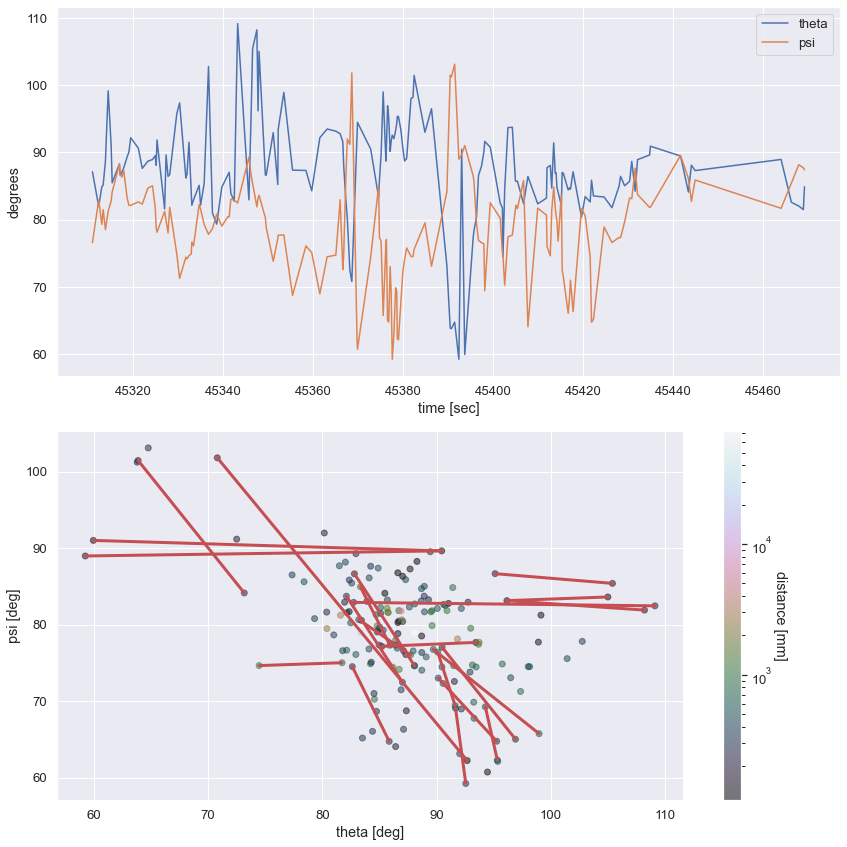
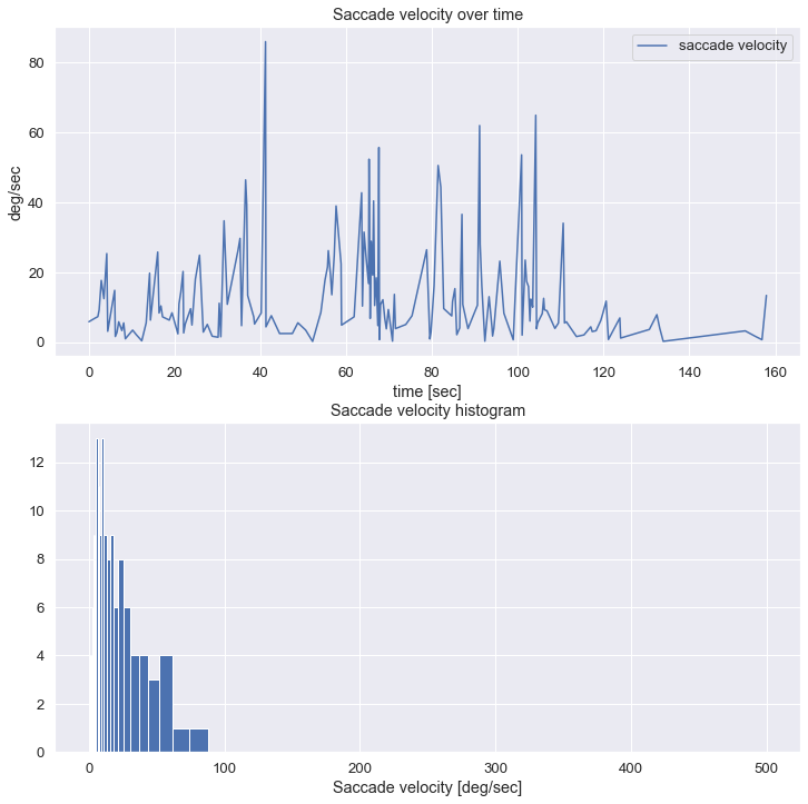
#5 - Visualizing Gaze Velocity
#Here we show how to visualize gaze velocity over time as well as the distribution of different velocities.
time = dataGaze.start_timestamp[:-1] - dataGaze.start_timestamp.iloc[0]
#sigma_theta = np.mean(dtheta_dt**2) - np.mean(dtheta_dt)**2
#sigma_psi = np.mean(dpsi_dt**2 ) - np.mean(dpsi_dt)**2
sigma_theta = np.sqrt(np.mean((dtheta_dt - np.mean(dtheta_dt))**2))
sigma_psi = np.sqrt(np.mean((dpsi_dt - np.mean(dpsi_dt ))**2))
eta_theta = lambda0*sigma_theta
eta_psi = lambda0*sigma_psi
tk = (dtheta_dt/eta_theta)**2 + (dpsi_dt/eta_psi)**2
idx = tk > 1
### number of saccades
nSaccade = np.sum(idx)
print('Number of saccades is ', nSaccade)
# getting density distribution vs. amplitude and fixation duration
amplitude = np.sqrt(theta**2 + psi**2)
### mean saccade speed
meanSpeed = 0
for i in range(len(idx) - 1):
if idx[i] == 1:
meanSpeed = meanSpeed + amplitude[i]
meanSpeed = meanSpeed/nSaccade
print('Mean saccade speed is ', meanSpeed, '(deg/s)')
##################### plots #####################
plt.figure(figsize=(12, 12))
plt.subplot(2, 1, 1)
sphere_pos_over_time(
dataGaze.start_timestamp,
data={"theta": theta, "psi": psi},
unit="degrees"
)
plt.subplot(2, 1, 2)
sphere_pos(r, theta, psi, unit="degrees")
for i in range(len(idx) - 1):
if idx[i] == 1:
plt.plot([theta[i], theta[i+1]], [psi[i], psi[i+1]], 'r', LineWidth = 3)
plt.tight_layout()
plt.figure(figsize=(12, 12))
plt.subplot(2, 1, 1)
sphere_pos_over_time(time, {"saccade velocity": deg_per_sec}, unit="deg/sec")
plt.title("Saccade velocity over time")
plt.subplot(2, 1, 2)
plt.hist(deg_per_sec, bins=np.logspace(-1, np.log10(500), 50))
plt.title("Saccade velocity histogram")
plt.xlabel("Saccade velocity [deg/sec]")
plt.figure(figsize=(12, 12))
plt.subplot(2, 1, 1)
plt.plot(dataGaze.gaze_point_3d_x, dataGaze.gaze_point_3d_y, 'y-o')
for i in range(len(idx) - 1):
if idx[i] == 1:
plt.plot([dataGaze.gaze_point_3d_x[i], dataGaze.gaze_point_3d_x[i+1]], [dataGaze.gaze_point_3d_y[i], dataGaze.gaze_point_3d_y[i+1]], 'r-+', LineWidth = 3)
plt.xlabel('x [minarc]')
plt.ylabel('y [min–arc]')
plt.subplot(2, 1, 2)
amp_cums = np.cumsum(amplitude)
velo_deg = np.sqrt(dtheta_dt**2 + dpsi_dt**2)
for i in range(len(idx) - 1):
if idx[i] == 1:
plt.loglog(np.cumsum(amp_cums[i]), velo_deg[i], 'ko')
plt.xlabel('amplitude(deg)')
plt.ylabel('Velocity')
plt.figure(figsize = (12, 12))
kde = stats.gaussian_kde(np.array(amplitude))
Z = kde(amplitude)
plt.plot(Z)
plt.title('Density vs. amplitude')
plt.xlabel('amplitude(deg)')
plt.ylabel('Density')
After we run the above script, we now have printed the number of saccades and saccade mean velocity in python console and we also plotted some graphs (see below).